Hello everyone, I’ve just released version 3 of Everything Will Be IK, my Inverse Kinematics library for Java (and the associated Processing implementation).

The library requires minimal expertise, and supports the following highly coveted features.
- Position AND orientation targets (6 degrees of freedom).
- Multiple end-effector support
- Multiple Intermediary-effector support.
- Dampening (to allow for a tradeoff between “naturalness” of the resulting pose, and speed of convergence).
- Target weight/priority (per target, per degree of freedom).
- Highly versatile 3 degree of freedom joint constraints with arbitrarily shaped orientation regions.
- Excellent stability under even extreme contortion (or, if speed is more important to you, merely extremely good stability in all but the most extreme cases)
This version includes the following improvements over version 2:
- Massive performance improvements. The example in the video above (which solves for 16 bones attempting to satisfy the orientations and positions of 4 effector-target pairs takes less than a tenth of a millisecond per iteration)
- More intuitive/predictable inputs for target orientations / position weights.
- A ton more examples and a much nicer visualizer.
You should be able to easily install the library directly from the processing IDE, by navigating to
- Tools->Add Tool
- Selecting the “Libraries” tab
- Searching “Everything Will be IK” and selecting the result.
- Clicking “Install”
- Restarting the Processing IDE
Once installed, a number of demos / examples (including the one in the video above) will appear under the new “Everything Will Be IK” heading of the “Contributed Libraries” section of the Processing IDE’s Examples tool. (Which you can access by navigating to File->Examples). All examples come in Double and Single Precision flavors. Double Precision is recommended for accuracy and speed (due to how Java’s trig libraries work, double appears to be faster than float), while Single Precision is recommended if you prefer working with native PVectors instead of the purpose-built “DVectors”.
If you prefer a more linear tutorial over a bunch of examples, I’ve included one below, which assumes you’ll be using the single precision variant for simplicity:
Basic Usage:
0: Open up the Single Precision flavor of the included “Learning Template” example. This template just imports the necessary libraries and some visualization code so we can see what we’re doing.
1: To start, you’ll need to define an armature (which is a container for a hierarchical collection of bones). Normally, you do this by declaring something like
Armature armature = new Armature();
The Learning Template has already declared one for us called simpleArmature, and already set it up to work nicely with the visualizer, so for the rest of this tutorial, we’ll just be adding our Bones to that one.
2: Every instance of an Armature comes with a default root bone already initialized. You build your Armature by adding Bones to this root bone, or to descendants of this root bone. So, first, let’s get a reference to the Armature’s root Bone by adding the following code to the end of the setup() function.
Bone rootBone = simpleArmature.getRootBone();
3: Next, let’s add a sequence of Bones to our root bone. The Bone class has a constructor of the form Bone(parentBone, boneName, boneHeight). Using this constructor, the Bones we declare will automatically attach themselves to the parentBone we specify. So we’ll create our chain by creating a Bone called initialBone , and setting rootBone as its parent. Then creating a Bone called secondBone , and setting initialBone as its parent. Then a Bone called thirdBone , using secondBone as its parent, and so on…
initialBone = new Bone(rootBone, "initial", 74f);
secondBone = new Bone(initialBone, "nextBone", 86f);
thirdBone = new Bone(secondBone, "anotherBone", 98f);
fourthBone = new Bone(thirdBone, "oneMoreBone", 70f);
fifthBone = new Bone(fourthBone, "fifthBone", 80f);
4: At this point, we’ve created a chain of 5 bones of varying heights. We haven’t constrained them yet, but we’ve done enough to test the IK solver. To try it out, we’ll first “pin” the rootBone to a position in space, then we’ll “pin” the fifthBone to its current position in space.
rootBone.enablePin();
fifthBone.enablePin();
Note “pin” here is library specific jargon for a target-effector pair. In more common parlance, an “effector” is a bone which attempts to reach a “target”.
5: Finally, for visualization purposes, let’s let the UI code know about our new pins so we can easily interact with them. Just add
ui.updatePinList(simpleArmature);
To the end of the setup function and you’re good to go.
Your complete setup function should now look like this.
public void setup() {
  size(1200, 900, P3D);
  simpleArmature = new Armature("example");
  setupVisualizationParams(simpleArmature);
  //USER CODE GOES BELOW THIS LINE:

  Bone rootBone = simpleArmature.getRootBone();
  Bone initialBone = new Bone(rootBone, "initial", 74f);
  Bone secondBone = new Bone(initialBone, "nextBone", 76f);
  Bone thirdBone = new Bone(secondBone, "anotherBone", 65f);
  Bone fourthBone = new Bone(thirdBone, "oneMoreBone", 70f);
  Bone fifthBone = new Bone(fourthBone, "fifthBone", 60f);

  rootBone.enablePin();
  fifthBone.enablePin();

  ui.updatePinList(simpleArmature);
}
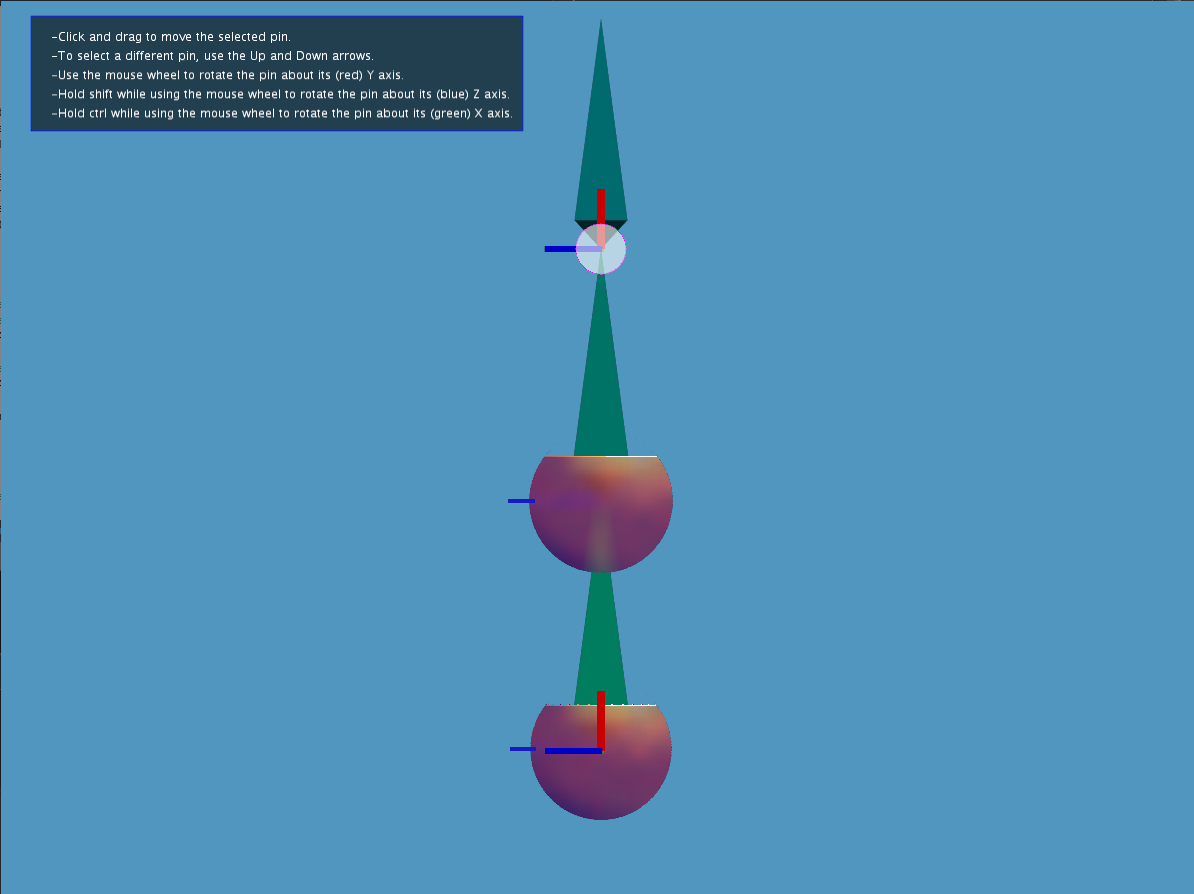
6: If you run the sketch, you should now see and be able to interact with something like this

Those two red/green/blue things on the first and last bones are our “pins,” right where we put 'em. You can move them around or rotate them as per the instructions on the top left of the screen, and the chain of bones will try its darndest to make sure each pinned bone reaches its target.
7: Right now, the draw() function and UI class are taking care of moving the pins in accordance with your mouse and keyboard input with the lines
if(mousePressed) {
   activePin.translateTo(new PVector(ui.mouse.x, ui.mouse.y, activePin.getLocation_().z));

    //THIS FUNCTION TELLS THE ARMATURE RUN THE IK SOLVER
	simpleArmature.IKSolver(simpleArmature.getRootBone());
}
But if you want to move them programmatically, all you would need to do is get a reference to the pin you want to modify, and translate or rotate it to the desired position and/or orientation, and then tell the armature to solve for the modified target.
For example, try adding the following lines to the end of your setup() function and running the sketch again to see this in action!
IKPin fifthBonePin = fifthBone.getIKPin();
fifthBonePin.translateTo(new PVector(200, 100, 0));
fifthBonePin.rotateAboutX(PI/2f);
simpleArmature.IKSolver(rootBone);
Seasoning To Taste:
0: You might notice that if you wiggle the target around really fast, the chain ends up looking sort of unnaturally scrunched. It’s still technically a valid solution, but not a very pretty one.

1: To mitigate this, we can lower the solver’s “dampening” parameter, which gives us a more natural look. Basically, all dampening does is limit how much each bone is allowed to rotate per solver iteration, in effect more evenly distributing the bend along the bone chain. Adding the line below to the setup function will set the maximum rotation per iteration to 0.001 radians.
simpleArmature.setDefaultDampening(0.001f);
2: This has the desired effect, but also takes quite longer to solve. To make it snappier, we can increase the number of iterations the IK solver runs per call. The default is 10, but something like 300 should do the trick.
simpleArmature.setDefaultIterations(300);
3: That’s much better. But do note that the greater the number of iterations you set, the higher the performance cost. It scales linearly, so if 30 iterations per call takes your processor 0.5ms, you can expect 300 iterations to take it 5ms. You’re encouraged to play around with these settings and figure out the ones that work best for your usecase. You can enable the built in performance monitor to help you get a sense of the cost of the computation by setting.
simpleArmature.setPerformanceMonitor(true);
The output will be printed to the processing console every second or so that you interact with the armature.
Setting Constraints:
1: While the above examples might be fun to play with, they are more or less trivial. What most people really want in an Inverse Kinematics library is one that can deal with the more realistic situation of joints that can only bend so much. In other words joint constraints. If you’ve shopped around for Inverse Kinematics libraries before, or maybe even tried to roll your own, you may have started to despair of ever finding one that handles these well. Don’t worry. You can finally relax. Eveything Will be IK … handles these wonderfully.
2: You can specify your joint limits through a novel system I call Kusudamas. It’s a bit difficult to explain in words how these work, but luckily, since a picture is worth a thousand words, the video below should help explain at 24,000 words per second.

Basically, you specify a sequence of points on a sphere. Each of these points has a radius – in essence making each define a cone with its tip at the center of the constraint (aka, the origin of the bone being constrained). The path that runs through this sequence of cones (widening and narrowing to meet the radius on each cone along the sequence) defines the region of directions each bone is allowed to point.
The directions these cones open toward are defined as vectors emanating from the base of the bone being constrained, defined in the coordinates of the parent of the bone being constrained. Such that a cone defined as (0, 1, 0) points directly away from the parent of the bone being constrained, while a cone defined as (-1, 0, 0) points perpendicular to the parent of the bone being constrained.
3: This sounds complicated, but it’s actually quite easy if you try. So let’s try with a fresh sketch so we can have a better look.
public void setup() {
  size(1200, 900, P3D);
  simpleArmature = new Armature("example");
  setupVisualizationParams(simpleArmature);
  //USER CODE GOES BELOW THIS LINE:

  Bone rootBone = simpleArmature.getRootBone();
  Bone initialBone = new Bone(rootBone, "initial", 124f);
  Bone secondBone = new Bone(initialBone, "nextBone", 126f);
  Bone thirdBone = new Bone(secondBone, "anotherBone", 115f);

  rootBone.enablePin();
  thirdBone.enablePin();

//CONSTRAINT CODE STARTS HERE:
 Bone.setDrawKusudamas(true);//tell all Bone objects to draw any constraints set on them.

 Kusudama b1Constraint = new Kusudama(initialBone); //define a Kusudama on the "initialBone"
 b1Constraint.addLimitConeAtIndex
             (0, //add our zeroeth Limit Cone
              new PVector(0, 1, 0), //pointing in the direction of (0, 1, 0)
              0.9f //with a "radius" (aka half-angle) of 0.9 radians
             );

 //do the same for the "secondBone"
  Kusudama b2Constraint = new Kusudama(secondBone);
  b2Constraint.addLimitConeAtIndex(0, new PVector(0, 1, 0), 0.9f);

  ui.updatePinList(simpleArmature);
}
Which should give us something that looks like this:
(Note how while interacting with the armature, neither of the bones that we constrained go outside of the purple spheres, regardless of where we set our targets.)
Note also how the center of the open portion of the constraints on each bone always points away from the parent of the bone it’s constraining. That’s because we set the limit cone vector to (0,1,0), and since the constraint is defined in terms of the parent bone’s transformation, and every bone is defined as pointing in the direction of its own transformation’s y-axis.
4: Now let’s try adding more cones to each Kusudama’s cone sequence. We’ll add a cone on the initialBone’s Kusudama pointing in the x direction, and one on the secondBone’s Kusudama pointing in the z direction.
  Kusudama b1Constraint = new Kusudama(initialBone);
  b1Constraint.addLimitConeAtIndex(0, new PVector(0, 1, 0), 0.9f);
  b1Constraint.addLimitConeAtIndex(1, new PVector(1, 0, 0), 0.3f);

  Kusudama b2Constraint = new Kusudama(secondBone);
  b2Constraint.addLimitConeAtIndex(0, new PVector(0, 1, 0), 0.9f);
  b2Constraint.addLimitConeAtIndex(1, new PVector(0, 0, 1), 0.3f);
Which should give us something like this.

And there’s no reason to stop there. You can define all sorts of crazy useless bounding regions which I just realized the shader apparently doesn’t visualize (I’ll fix it next update), but regardless they do work and the solver does respect them.
5: Now that we have the orientation constraints defined, all that’s left is to define the axial limits. That is to say, how much each bone is allowed to “twist” relative to its parent bone. This is visualized in the video above and the included shader by that little fan thing sticking out of the purple sphere. The blue line within the fan indicates the Bone’s z-axis, and the fan itself sets boundaries on how much the z-axis is allowed to deviate from the z-axis of the parent bone if you were to rotate the bone back to point in the same direction as its parent by the shortest rotation possible.
Setting these is as simple as adding
b1Constraint.setAxialLimits(
   -0.3f, //floor of allowable twist
   0.3f //ceiling of allowable trist
 ,);
Happy Hacking!
Those are all the tidbits you need to get started! Poke around the included examples to get a sense of what else is possible. Or take a gander at the included reference docs, or just a drop a question here! Bug reports, suggestions, and feature requests welcome ![]()
