Understanding the Diffusion Curves Algorithm

[micycle]

Paper outcome above. I’m not going anything this complicated (beziers) yet, but just a simple working prototype of the diffusion part.

---

The broad idea with Diffusion Curves is you specify some pixels in a canvas (such as the colour bezier lines in (b) above) and then spread the colours throughout the rest of the canvas by, for each pixel, averaging the four adjacent (non-diagonal) pixels (i.e. up, down, left, right). This is repeated until all the pixels are filled and the colours stabilise.

With that brief introduction, my question concerns section 3.2.2 of this paper.

There’s a lot maths leading up to this part, but the diffusion algorithm seems to boil down to something quite simple:

So, if a pixel (at location i,j) is user-defined (alpha-mask > 0), you don’t average it with other pixels – rather, you keep the user-defined colour. Otherwise, you average a pixel with it’s neighboring pixels.

But it’s the formula of this averaging part that is a bit confusing:

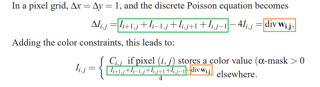
divw_ij is first defined as the green region minus 4I_ij. However, in the next part (which tells us how to calculate a pixel), divw_ij is subtracted from the green region, essentially cancelling out each value, leaving only positive 4I_ij – this has to be wrong, so my question is: what’s going on here?

---

Another point of confusion: straight after that divw_ij is (re)defined as this:

.
I’m not sure whether I’m meant to do anything with that😁.

---

Appendix: the loop I’ve developed so far simply averages the neighboring pixels and kinda works, but it’s not quite implementing the paper.

for (int x = 1; x < width - 1; x++) { // -1 edge buffer
	for (int y = 1; y < height - 1; y++) {
		
		if (alphaMask[x][y] == 1) { // dont diffuse user-defined pixels
			pixels[x + width * y] = composeclr(canvas[x][y]);  // but still copy user-defined pixel into pixels[]
			continue;
		}
		
		canvas[x][y][0] = // R component
				0.25f * canvas[x - 1][y][0] + 
				0.25f * canvas[x + 1][y][0] + 
				0.25f * canvas[x][y - 1][0] + 
				0.25f * canvas[x][y + 1][0];
		canvas[x][y][1] = // B component
				0.25f * canvas[x - 1][y][1] + 
				0.25f * canvas[x + 1][y][1] + 
				0.25f * canvas[x][y - 1][1] + 
				0.25f * canvas[x][y + 1][1];
		canvas[x][y][2] = // B component
				0.25f * canvas[x - 1][y][2] + 
				0.25f * canvas[x + 1][y][2] + 
				0.25f * canvas[x][y - 1][2] + 
				0.25f * canvas[x][y + 1][2];

		pixels[x + width * y] = composeclr(canvas[x][y]); // write int clr into Processing pixels[]
	}

Input: 2000 random-coloured pixels

Input: One-pixel high pink and blue lines

[micycle]

Another paper more plainly states how to derive the colour of a pixel from its neighbours at each iteration:

… which more-or-less accords with how I implemented the code before.

So I then looked at the previous paper from my first post closely: it defines ∆I_i,j first, and then defines I_i,j. Notice there’s no delta – they’re different!

divw_i,j is actually the “the divergence of the gradient (w)” at w_i,j. It seems that this is used to find a cleaner boundary between colours (which are rasterized as bezier curves in the paper). See below:

Now the last equation I highlighted in my previous post is comprehensible: this divw_i,j, is calculated for a pixel by calculating the mean of the gradients of the surrounding pixels (in the x and y directions). However, it can be omitted for my more simpler purposes (for the moment at least).

---

Also, it turns out that I was referencing the above and below pixels incorrectly in my code. I was referencing the pixel above as [x-1][y+1], when it should have been [x][y+1]; and referencing the pixel below as [x+1][y-1], when it should have been [x][y-1]… That’s why the colour spread was skewed at a 45° angle – I knew something was up with it!

Another problem with my code was that it was using the new value of a pixel from the current iteration in the calculation of the next pixel, rather than referencing values from the previous iteration only. An output of the corrected code is below:

Now to work on the “multigrid” part of the algorithm!..

[seanc4s]

You could apply a simple 2D binomial filter a few times, maybe?
http://www.cse.yorku.ca/~kosta/CompVis_Notes/binomial_filters.pdf.old

You can do the simple 1D [1,2,1] filter a number of times alternately across all the horizontal lines in the image and then all the vertical lines, then all the horizontal lines again…

[jeremydouglass]

Is the point of implementing multigrid that it produces the same output, but much more efficiently?

It seems like that approach would only work with images whose dimensions are powers of two.

[micycle]

apply a simple 2D binomial filter a few times, maybe

… as the filter to apply before downsampling? That’s what the paper suggests!

[micycle]

@jeremydouglass

Is the point of implementing multi-grid that it produces the same output, but much more efficiently?

Yeah, exactly. The kernel approach (Jacobi iteration) converges very slowly. To illustrate, in a given direction we propagate only 25% of a filled-in pixel to the adjacent pixel in one iteration. Doing this across thousands of pixels? Yeah… It’s going to take a while for the further-most pixel to even begin being filled in…

I think the intuition of the multi-grid approach is best exemplified by comparing the 512x512 with the 16x16 after 5 rounds of down-sampling:

We see that the colour takes up a much larger proportion of the 16x16 image. Notably, if this were to be scaled up with nearest-neighbour, that proportion would remain.

Jacobi iterations at the 16x16 resolution spreads the colour to the edges of image almost immediately (albeit low frequency information). When this coarse solution is then up-sampled with nearest-neighbour, each pixel may not have the exact colour, but it has a close colour, giving it a huge jump-start in the convergence process. And now, rather than expending so many iterations propagating colour to the outermost pixels, we simply need to refine the coarse colour (using far fewer iterations).

[jeremydouglass]

Thanks! Is this something that you are thinking about implementing as a PShader?

[micycle]

Not yet, at least. I’m still a beginner when it comes to shaders.

[jeremydouglass]

@micycle

When this coarse solution is then up-sampled with neighbor

Interesting. Do you then upsample straight from 16x16 to 512x512 before continuing to propagate? Or do you upsample / propagate / upsample / propagate from 16x, 32x, 64x, 128x, 256x?

[micycle]

From the paper:

Typically, for a 512×512 image we use 5i Jacobi iterations per multigrid level, with i the level
number from fine to coarse.

So downsample (with a binomial-like kernel) all the way down and then: iterate—>upsample repeat.

Right now though, I’m having problem figuring out whether/how to use the alpha grid as I iterate after upscaling, since these exact details don’t seem to be given in the paper.

[jeremydouglass]

Got it. I’m imagining something like this (untested pseudocode):

int MGMAX = 9;  // 2^9 = 512
int MGMIN = 4;  // 2^4 = 16
int UPSCALE_PROPS = 5;  // magic number

// ...

class Diffuser {

  // ...

  void multigrid() {
    for(int i=MGMAX; i>MGMIN; i--) {
      this.downscale();
    }
    this.jacobiUntilStable();
    for(int i=MGMIN; i<MGMAX; i++) {
      this.upscale();
      for(int j=0; j<UPSCALE_PROPS; j++) {
        this.jacobiStep(); 
      }
    }
    this.jacobiUntilStable();
  }
}

[micycle]

Yeah, that’s it (j might start at 1 though…).

[micycle]

I’ve managed to implement the multigrid approach.

Code (high level)

final int LEVELS = 5; // multigrid levels
final int JACOBI = 15; // jacobi ierations

ImageArray imgArray = new ImageArray(pixels, mask);

for (int i = 0; i < LEVELS; i++) {
	MultiGrid.filterImage(imgArray); // apply 3x3 kernel
	MultiGrid.downsampleImage(imgArray);
}

for (int i = 0; i < LEVELS; i++) {
	for (int j = 0; j < JACOBI; j++) {
		MultiGrid.diffuseImage(imgArray);
	}
	MultiGrid.upscaleImage(imgArray); // nearest neighbour upscale
}
for (int j = 0; j < JACOBI; j++) { // diffuse after final upscale 
	MultiGrid.diffuseImage(imgArray);
}

One thing left to do is iterate the edges of the pixels at each level in the down/upscale, diffusion and filter, so I’m not left with black (empty) edges which are not diffused/upscaled into.

Another thing (that’s not clear from the paper) is how to set the pixel mask for the next lot of diffusion iterations following an upscale. (The mask effects whether pixels can be diffused into (given a new value based on surrounding pixels), or not (retain their colour after the upscale and be read-only)).

So I’ve experimented with a few approaches, but none of the results quite match the output in the paper (retaining the original pixels with diffusion elsewhere, like the image in one of my previous posts). My only other thought is to save the original mask at each level during the downscale and use those exacts masks at each corresponding level in the upscale.

The upscaling is simply nearest neighbour, like below:

…so in the following images, I show the effect of changing which (if any) of the 4 upscaled pixels gets masked after an upscale.

The following images show output after 6 multigrid levels with 15 diffusion iterations at each level:

Input

Output (mask the bottom-left-most upscaled pixel)

Gets a bit blobby in certain places because those pixels have been repeatedly masked – in other words, never diffused.

Output (no mask after upscale, all pixels diffused)

Very blurry since we are diffusing every pixel every time.

Output (randomly mask 1 of the 4 upscaled pixels)

Rather than always choosing the bottom-left-most pixel, choose it randomly Serendipitously, this has a watercolour-like effect.

Output (mask every pixel, no pixels diffused)

Simply repeated nearest-neighbour upscaling

[micycle]

When using the pixel mask created for each layer (when downscaling) for the diffusion at each level in the upscale, original lines are preserved and the unwanted blobby effect seen previously disappears.

>

>

However, whenever different-coloured lines meet (or are close), an artifact is introduced.

Not sure why this is…

A better example: many lines crossing

>

Becomes rather blocky…

>

Played around with the diffusion equation and got some funky results:

>